10: Statistical analysis

A recent sentiment analysis study presents a comprehensive breakdown of emotions in a dataset, revealing a stark dominance of neutrality in the discourse examined. The donut chart illustrates the sentiment distribution, showcasing that a whopping 73.9% of the entries maintained a neutral tone.

Emotion Recognition and Sentiment Analysis

import pandas as pd
import plotly.express as px
import plotly.graph_objects as go

# Load the dataset
data = pd.read_csv('main.csv')

# Create a bar graph for emotions using Plotly
emotion_counts = data['emotion'].value_counts().reset_index()
emotion_counts.columns = ['emotion', 'count']
fig_bar = px.bar(emotion_counts, x='emotion', y='count', title='Distribution of Emotions',
                 labels={'count': 'Count', 'emotion': 'Emotion'}, color='emotion',
                 color_continuous_scale=px.colors.sequential.Viridis)
fig_bar.update_layout(xaxis_title='Emotion', yaxis_title='Count', showlegend=False)
fig_bar.show()

# Create a donut chart for sentiment using Plotly
sentiment_counts = data['sentiment'].value_counts().reset_index()
sentiment_counts.columns = ['sentiment', 'count']
fig_donut = px.pie(sentiment_counts, values='count', names='sentiment', title='Distribution of Sentiments',
                   hole=0.4, color='sentiment', color_discrete_sequence=px.colors.sequential.RdBu)
fig_donut.update_traces(textposition='inside', textinfo='percent+label')
fig_donut.show()

Relationship between Sentiment and Emotion Confidence Scores The plot likely represents the confidence levels of sentiment and emotion predictions, with each point color-coded by sentiment category. The spread and clustering of points can help assess the precision of your sentiment analysis models and identify which emotions or sentiments are predicted with more confidence, providing insights into the reliability of different aspects of your sentiment analysis framework.

import pandas as pd
import plotly.express as px

# Load the dataset
data = pd.read_csv('main.csv')

# Histogram of Sentiment Confidence Values
fig_hist_sentiment = px.histogram(data, x='sentiment_score', color='sentiment',
                                  title='Distribution of Sentiment Confidence Scores',
                                  labels={'sentiment_score': 'Confidence Score'},
                                  opacity=0.8)
fig_hist_sentiment.show()

# Scatter Plot of Sentiment vs Emotion Confidence
fig_scatter = px.scatter(data, x='sentiment_score', y='emotion_score', color='sentiment',
                         title='Relationship between Sentiment and Emotion Confidence Scores',
                         labels={'sentiment_score': 'Sentiment Confidence', 'emotion_score': 'Emotion Confidence'})
fig_scatter.show()

Confidence Scores Distribution for Each Emotion This boxplot distribution shows the variability and central tendency of confidence scores across different emotions. It helps in evaluating the consistency of emotion recognition models, revealing which emotions are recognized with higher confidence and which may require further model tuning or training on more diverse datasets.

import pandas as pd
import plotly.express as px

# Load the dataset
data = pd.read_csv('main.csv')
# Box Plot for Emotion Confidence by Emotion Category
fig_box = px.box(data, x='emotion', y='emotion_score', color='emotion',
                 title='Confidence Scores Distribution for Each Emotion',
                 labels={'emotion_score': 'Emotion Confidence', 'emotion': 'Emotion'})
fig_box.update_traces(quartilemethod="inclusive")  # or "exclusive", depending on how you want to calculate quartiles
fig_box.show()

Classification LSTM Model

Initial Model: Multinomial Naive Bayes

from sklearn.feature_extraction.text import TfidfVectorizer
from sklearn.preprocessing import OneHotEncoder
from sklearn.compose import ColumnTransformer
from sklearn.pipeline import Pipeline
from sklearn.naive_bayes import MultinomialNB
from sklearn.model_selection import train_test_split
from sklearn.metrics import classification_report


# Data loading and preprocessing
df = pd.read_csv('main.csv')
df = df[['TITLE', 'sentiment', 'emotion','ARTICLE', 'AUTHOR']]

# Column Transformer to handle different feature types
preprocessor = ColumnTransformer(
    transformers=[
        ('tfidf1', TfidfVectorizer(stop_words='english'), 'TITLE'),
        ('tfidf2', TfidfVectorizer(stop_words='english'), 'ARTICLE'),
        ('onehot', OneHotEncoder(), ['sentiment', 'emotion'])
    ])

# Pipeline to vectorize text and train model
pipeline = Pipeline([
    ('preprocessor', preprocessor),
    ('classifier', MultinomialNB())
])

# Training and prediction

Second Model: Logistic Regression

from sklearn.feature_extraction.text import TfidfVectorizer
from sklearn.preprocessing import OneHotEncoder
from sklearn.compose import ColumnTransformer
from sklearn.pipeline import Pipeline
from sklearn.naive_bayes import MultinomialNB
from sklearn.model_selection import train_test_split
from sklearn.metrics import classification_report
from sklearn.linear_model import LogisticRegression


df = pd.read_csv('main.csv')
df = df[['TITLE', 'sentiment', 'emotion','ARTICLE', 'AUTHOR']]

# Column Transformer to handle different feature types
preprocessor = ColumnTransformer(
    transformers=[
        ('tfidf1', TfidfVectorizer(stop_words='english'), 'TITLE'),
        ('tfidf2', TfidfVectorizer(stop_words='english'), 'ARTICLE'),
        ('onehot', OneHotEncoder(), ['sentiment', 'emotion'])
    ])

# Pipeline to vectorize text and train model
pipeline = Pipeline([
    ('preprocessor', preprocessor),
    ('classifier', LogisticRegression(C=1.0, random_state=42))
])

# Training and prediction

Final Model: LSTM Neural Network

import tensorflow as tf
import pandas as pd
import numpy as np
from tensorflow.keras.layers import Input, Embedding, LSTM, Dense, Concatenate
from tensorflow.keras.models import Model
from tensorflow.keras.preprocessing.text import Tokenizer
from tensorflow.keras.preprocessing.sequence import pad_sequences
from sklearn.preprocessing import LabelEncoder
from tensorflow.keras.callbacks import EarlyStopping
from tensorflow.keras.callbacks import TensorBoard
from sklearn.model_selection import train_test_split

df=pd.read_csv('main.csv')
# Prepare your data
df=df[["AUTHOR","TITLE","sentiment","emotion","ARTICLE"]]
tokenizer = Tokenizer(num_words=1000, oov_token="<OOV>")
tokenizer.fit_on_texts(df['TITLE'])
title_sequences = tokenizer.texts_to_sequences(df['TITLE'])
title_padded = pad_sequences(title_sequences, maxlen=50)

tokenizer = Tokenizer(num_words=1000, oov_token="<OOV>")
tokenizer.fit_on_texts(df['ARTICLE'])
art_sequences = tokenizer.texts_to_sequences(df['ARTICLE'])
art_padded = pad_sequences(art_sequences, maxlen=500)

# One-hot encode sentiment and emotion
sentiment_encoded = pd.get_dummies(df['sentiment']).values
emotion_encoded = pd.get_dummies(df['emotion']).values

# Concatenate all features
import numpy as np
features = np.concatenate([title_padded, sentiment_encoded, emotion_encoded,art_padded], axis=1)

# Model building
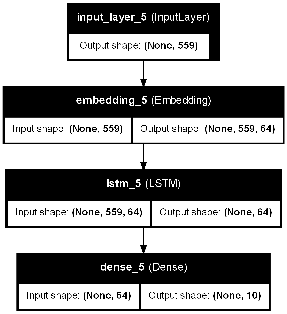
input_layer = Input(shape=(features.shape[1],))
embedding = Embedding(input_dim=1000, output_dim=64, input_length=features.shape[1])(input_layer)
lstm_layer = LSTM(64)(embedding)
output_layer = Dense(len(df['AUTHOR'].unique()), activation='softmax')(lstm_layer)
model = Model(inputs=input_layer, outputs=output_layer)

model.compile(optimizer='adamax', loss='sparse_categorical_crossentropy', metrics=['accuracy'])
early_stopping = EarlyStopping(monitor='val_accuracy', patience=10, restore_best_weights=True)
#tensorboard_callback = TensorBoard(log_dir="./logs")

# Model training
labels = LabelEncoder().fit_transform(df['AUTHOR'])
X_train, X_test, y_train, y_test = train_test_split(features, labels, test_size=0.3, random_state=42)
history=model.fit(X_train, y_train, epochs=100, validation_data=(X_test, y_test),callbacks=[early_stopping])

Comprehensive Input Features: The model leverages a variety of input features including titles and articles, which are tokenized and padded to uniform lengths. Sentiment and emotion are also encoded as additional features, suggesting a multidimensional approach to understanding text data.

Use of LSTM Layer: The LSTM (Long Short-Term Memory) layer is pivotal for processing sequences in the text, capturing temporal dependencies that might be crucial for predicting the author based on writing style and content nuances.

Embedding Layer: The inclusion of an Embedding layer indicates an effort to transform tokenized words into dense vectors of fixed size, likely aiding in the effective representation of words in a lower-dimensional space.

Output Layer: The Dense layer with a softmax activation function maps the LSTM outputs to probabilities across the different authors, facilitating multi-class classification.

Optimizer and Loss Function: The model uses the ‘adamax’ optimizer and ‘sparse_categorical_crossentropy’, which are suitable choices for multi-class classification problems involving categorical label encoding.

Early Stopping: Implementation of Early Stopping to prevent overfitting by halting the training process if the validation accuracy does not improve for consecutive epochs, ensuring the model generalizes well on unseen data.

Validation Split: The use of a 30% validation split helps in monitoring the model’s performance on a separate set of data that was not used during training, which is crucial for assessing the generalization capability of the model.

Neural Network Results

Model Plot

Model Plot

Model Loss

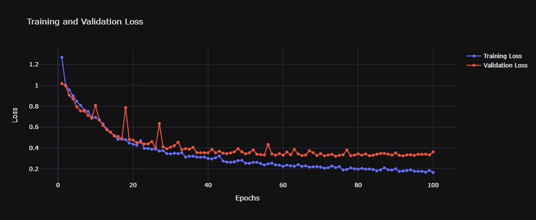
Model Training and Validation Loss

Model Accuracy

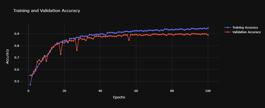
Model Training and Validation Accuracy

Prediction Matrix

Model Training and Validation Accuracy

High Accuracy: The model achieves a commendable accuracy of 89.2%, indicating strong predictive performance. This suggests that the features and LSTM architecture effectively capture the characteristics necessary to distinguish between authors.

Visualization Tools: The inclusion of plots such as the model loss, accuracy, and a confusion matrix provides visual feedback on training dynamics and classification performance, aiding in quick assessment and iterative improvements.

Loss and Accuracy Trends: From the provided plots, one can discuss trends observed in training and validation loss and accuracy, noting any signs of overfitting or underfitting, and how early stopping may have intervened.